

Biden’s Approval Margins
In this post, we will use data from <www.fivethirtyeight.com> on all polls that track the president Biden’s approval rate in the US. (https://projects.fivethirtyeight.com/biden-approval-ratings)
Import data
# Import approval polls data directly off fivethirtyeight website
approval_polllist <- read_csv('https://projects.fivethirtyeight.com/biden-approval-data/approval_polllist.csv')

glimpse(approval_polllist)
## Rows: 1,597
## Columns: 22
## $ president <chr> "Joseph R. Biden Jr.", "Joseph R. Biden Jr.", "Jos~
## $ subgroup <chr> "All polls", "All polls", "All polls", "All polls"~
## $ modeldate <chr> "9/21/2021", "9/21/2021", "9/21/2021", "9/21/2021"~
## $ startdate <chr> "2/3/2021", "2/4/2021", "2/4/2021", "2/5/2021", "2~
## $ enddate <chr> "2/7/2021", "2/6/2021", "2/8/2021", "2/7/2021", "2~
## $ pollster <chr> "Rasmussen Reports/Pulse Opinion Research", "RMG R~
## $ grade <chr> "B", "B-", "B", "B", "B", "B", "B+", "B", "B+", "B~
## $ samplesize <dbl> 1500, 1200, 1500, 15000, 1986, 15000, 2508, 15000,~
## $ population <chr> "lv", "rv", "lv", "a", "rv", "a", "a", "a", "a", "~
## $ weight <dbl> 0.192, 0.881, 0.537, 0.265, 0.105, 0.239, 1.588, 0~
## $ influence <dbl> 0, 0, 0, 0, 0, 0, 0, 0, 0, 0, 0, 0, 0, 0, 0, 0, 0,~
## $ approve <dbl> 50.0, 60.0, 51.0, 55.0, 59.0, 55.0, 61.0, 55.0, 50~
## $ disapprove <dbl> 47.0, 32.0, 46.0, 33.0, 35.0, 33.0, 39.0, 33.0, 37~
## $ adjusted_approve <dbl> 52.5, 59.3, 53.5, 53.6, 57.6, 53.6, 62.3, 53.6, 51~
## $ adjusted_disapprove <dbl> 41.0, 33.1, 40.0, 36.3, 38.3, 36.3, 39.3, 36.3, 37~
## $ multiversions <chr> NA, NA, NA, NA, NA, NA, NA, NA, NA, NA, NA, NA, NA~
## $ tracking <lgl> TRUE, NA, TRUE, TRUE, NA, TRUE, NA, TRUE, NA, TRUE~
## $ url <chr> "https://www.rasmussenreports.com/public_content/p~
## $ poll_id <dbl> 74349, 74354, 74352, 74372, 74351, 74370, 74357, 7~
## $ question_id <dbl> 139669, 139679, 139675, 139746, 139673, 139738, 13~
## $ createddate <chr> "2/8/2021", "2/9/2021", "2/9/2021", "2/11/2021", "~
## $ timestamp <chr> "09:36:08 21 Sep 2021", "09:36:08 21 Sep 2021", "0~# Use `lubridate` to fix dates, as they are given as characters.
# Use enddate as the date of the poll result
approval_polllist <- approval_polllist %>%
mutate(enddate = mdy(enddate))Create a plot
Using the data, we wish to calculate the average net approval rate (approve - disapprove) for each week since Biden got into office. Then we would like to plot the net approval rate, along with its 95% confidence interval.
Tidy data and calculate Confidence Interval
#tidy data and calculate CI using formula.
net_approval <- approval_polllist %>%
  #We concentrate only on subgroup "voters"
  filter(!is.na(subgroup), subgroup == "Voters") %>%
  #Use lubridate to get week number
  mutate(week = isoweek(enddate),
         net_approval_day = approve - disapprove) %>%
  group_by(week) %>%
  summarise(mean_net_approval = mean(net_approval_day),
            sd_net_approval = sd(net_approval_day),
            count = n(),
            se_twitter = sd_net_approval / sqrt(count),
            t_critical = qt(0.975, count - 1),
            lower_ci =  mean_net_approval - t_critical*se_twitter,
            upper_ci = mean_net_approval + t_critical*se_twitter)

#Report the weekly net approval rate for Biden
net_approval %>%
  knitr::kable(bootstrap_options = c ("striped","hover","condensed","responsive")) %>%
kableExtra::kable_styling(font_size = 1)| week | mean_net_approval | sd_net_approval | count | se_twitter | t_critical | lower_ci | upper_ci |
|---|---|---|---|---|---|---|---|
| 5 | 18.333 | 13.43 | 3 | 7.75 | 4.30 | -15.026 | 51.69 |
| 6 | 10.889 | 6.90 | 9 | 2.30 | 2.31 | 5.585 | 16.19 |
| 7 | 13.000 | 9.16 | 14 | 2.45 | 2.16 | 7.713 | 18.29 |
| 8 | 11.044 | 8.85 | 15 | 2.29 | 2.14 | 6.142 | 15.95 |
| 9 | 7.545 | 6.88 | 11 | 2.07 | 2.23 | 2.926 | 12.16 |
| 10 | 9.583 | 7.46 | 12 | 2.15 | 2.20 | 4.841 | 14.33 |
| 11 | 11.833 | 9.95 | 12 | 2.87 | 2.20 | 5.510 | 18.16 |
| 12 | 9.231 | 10.36 | 13 | 2.87 | 2.18 | 2.969 | 15.49 |
| 13 | 6.300 | 9.67 | 10 | 3.06 | 2.26 | -0.620 | 13.22 |
| 14 | 6.625 | 9.47 | 8 | 3.35 | 2.37 | -1.293 | 14.54 |
| 15 | 8.933 | 7.52 | 15 | 1.94 | 2.14 | 4.771 | 13.10 |
| 16 | 10.067 | 7.97 | 15 | 2.06 | 2.14 | 5.654 | 14.48 |
| 17 | 9.346 | 10.07 | 13 | 2.79 | 2.18 | 3.259 | 15.43 |
| 18 | 8.233 | 7.60 | 12 | 2.19 | 2.20 | 3.405 | 13.06 |
| 19 | 3.500 | 5.18 | 8 | 1.83 | 2.37 | -0.833 | 7.83 |
| 20 | 12.821 | 7.23 | 14 | 1.93 | 2.16 | 8.646 | 17.00 |
| 21 | 12.385 | 5.99 | 13 | 1.66 | 2.18 | 8.763 | 16.01 |
| 22 | 7.111 | 7.69 | 9 | 2.56 | 2.31 | 1.201 | 13.02 |
| 23 | 7.091 | 7.05 | 11 | 2.12 | 2.23 | 2.355 | 11.83 |
| 24 | 8.643 | 7.22 | 14 | 1.93 | 2.16 | 4.476 | 12.81 |
| 25 | 7.030 | 4.79 | 10 | 1.51 | 2.26 | 3.605 | 10.46 |
| 26 | 6.400 | 7.91 | 10 | 2.50 | 2.26 | 0.745 | 12.05 |
| 27 | 6.200 | 8.13 | 10 | 2.57 | 2.26 | 0.381 | 12.02 |
| 28 | 2.375 | 3.62 | 8 | 1.28 | 2.37 | -0.654 | 5.40 |
| 29 | 6.400 | 5.28 | 10 | 1.67 | 2.26 | 2.627 | 10.17 |
| 30 | 2.429 | 7.92 | 14 | 2.12 | 2.16 | -2.144 | 7.00 |
| 31 | 3.583 | 6.23 | 12 | 1.80 | 2.20 | -0.375 | 7.54 |
| 32 | 1.000 | 6.42 | 11 | 1.94 | 2.23 | -3.312 | 5.31 |
| 33 | -0.267 | 5.66 | 15 | 1.46 | 2.14 | -3.403 | 2.87 |
| 34 | -7.090 | 5.85 | 10 | 1.85 | 2.26 | -11.272 | -2.91 |
| 35 | -5.700 | 5.70 | 13 | 1.58 | 2.18 | -9.144 | -2.26 |
| 36 | -3.986 | 3.75 | 14 | 1.00 | 2.16 | -6.153 | -1.82 |
| 37 | -5.143 | 5.07 | 14 | 1.35 | 2.16 | -8.068 | -2.22 |
| 38 | -3.500 | 12.02 | 2 | 8.50 | 12.71 | -111.503 | 104.50 |
Plot the net approval rate
ggplot(net_approval,
       aes(x= week,
           y= mean_net_approval)) +
  geom_line(color = "red")+
  geom_point(color = "red", size = 1)+
  geom_smooth(color = "blue",
              level = 0,
              size = 1)+
  #add orange line at zero
  geom_hline(yintercept=0,
             color = "orange",
             size = 2)+
  theme_minimal()+
  #add confidence band using calculated CI
  geom_ribbon(aes(ymin = lower_ci,
                  ymax = upper_ci),
              alpha=0.3,
              fill = "grey",
              color = "red") +
  labs(
    title = "Estimating Approval Margin (approve-disapprove) for Joe Biden",
    subtitle = "Weekly average approval of subgroup \"Voters\"",
    x = "Week of the year",
    y = "Average Approval Margin (approve-disapprove)")+
  scale_y_continuous(breaks=seq(-15,10,2.5), limits=c(-15,40))+
  scale_x_continuous(breaks=seq(0,40,13))+
  theme(
    axis.text.x = element_text(size = 18),
    axis.text.y = element_text(size = 18),
    axis.title.x = element_text(size=22, face="bold"),
    axis.title.y = element_text(size=22, face="bold"),
    plot.title = element_text(size = 22, face="bold"),
    plot.subtitle = element_text(size=20, face="bold")
  )+
   annotate("text", x=19.5, y=20, label="2021", color = "#333333", size=8)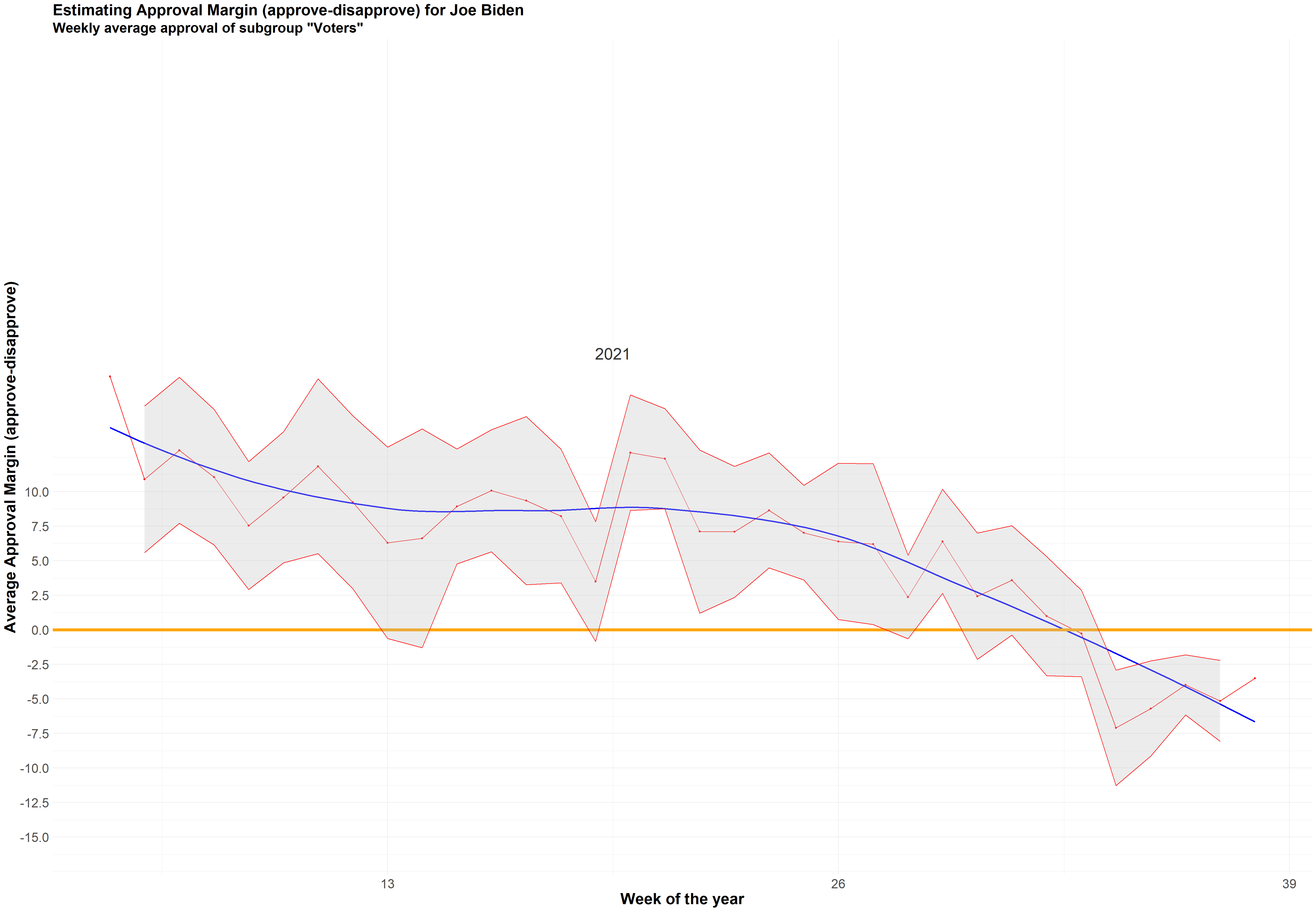
Compare Confidence Intervals
We then compare the confidence intervals for week 5 and week 25 to see if there are any changes in Biden’s net approval rate.
net_approval_5_25 <- net_approval %>%
  filter(week %in% c(5, 25)) %>%
  mutate(
    ci_width = upper_ci - lower_ci) %>%
  select(week, lower_ci, upper_ci, ci_width)

net_approval_5_25 %>%
  knitr::kable(bootstrap_options = c ("striped","hover","condensed","responsive")) %>%
kableExtra::kable_styling()| week | lower_ci | upper_ci | ci_width |
|---|---|---|---|
| 5 | -15.0 | 51.7 | 66.72 |
| 25 | 3.6 | 10.5 | 6.85 |
Analysis of the difference
From the results, we can clearly see that the confidence interval for Biden’s net approval rate has been narrower from week 5 to week 25.
The standard deviation in approval ratings is much larger in week 5 than in week 25, which generates a higher standard error and consequently a wider confidence interval. We assume this is because as after Biden has been elected for a longer period of time in week 25 (almost half a year), voters would become more clear about their approval or disapproval to the president. After Americans took over 25-week time to evaluate their newly elected president, they would probably have a clearer attitude towards Biden’s policy changes, administration and national strategies. These clearer perceptions then result in this decreasing variance in approval ratings, consequently a lower standard deviation and ultimately more narrow confidence intervals.